Mn/Model Final Report Chapter 8.16: Hardwood Hills

Quick Links

Chapters

Appendices

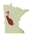
8.16 HARDWOOD HILLS SUBSECTION OF MINNESOTA & NE IOWA MORAINAL SECTION

8.16.1 Environmental Context
8.16.2 Site Probability Model
8.16.3 Survey Probability Model
8.16.4 Survey Implementation Model
8.16.5 Other Models

This regional model report is organized as described in Sections 8.2.1 through 8.4.1. Refer to these sections of the report for explanations of the tables, variables, and statistics.

8.16.1 Environmental Context

The Hardwood Hills is a subsection of the Minnesota and Northeast Iowa Morainal Section of the Eastern Broadleaf Forest Province (Figure 8.1) (Minnesota DNR 1998). This area is characterized by numerous kettle lakes on moraine and outwash deposits.

The eastern limits of Glacial Lake Agassiz deposits and the ice contact sediments of the Des Moines Lobe define the northern portion of the western boundary. The southern portion of the western boundary is defined by the interface between Des Moines Lobe moraines and the Alexandria moraine complex. The historical interface between the Big Woods and jack pine, white pine/red pine, or aspen-birch woodlands delimit the northeastern border. The southeastern boundary is defined by the interface between Mississippi valley outwash and the Wadena Lobe stagnation moraine (Dan Hanson, personal communication 1997).

The ground, end, and stagnation moraines that occupy most of this subsection are interrupted by areas of outwash (Figure 8.16.2.a). The topography varies from gently rolling to rugged. The continental divide separates this subsection into northern and southern halves. The drainage reflects this, with streams in the north flowing to the Red River, and the streams in the south flowing to the Mississippi River (Figure 8.16.1.a). Lakes are numerous and occur on both moraines and outwash material (Minnesota DNR 1998). Soils are mostly well-drained. However, poorly drained soils tend to occur in areas of ground moraine (Figure 8.16.2.a and b).

Irregular topography and the presence of lakes and wetlands provided some protection from fire in this subsection. This resulted in a complex pattern of prairie, oak woodlands, and Big Woods historic vegetation (Figure 8.16.1.b). In general, prairie is to the south and west and Big Woods to the east, with oak openings and barrens between them. Prairie tended to occupy more level terrain, with Big Woods in areas protected from the spread of fire by rugged relief or water bodies.

Return to Top

8.16.2 Site Probability Model

8.16.2.1 Description

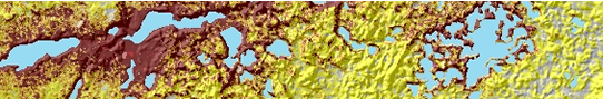
Zones of high and medium site potential are located primarily around lakes or chains of lakes in the site probability model (Figure 8.16.3). The largest contiguous areas of high and medium site potential are found around the scores of lakes in Douglas County and in northern Kandiyohi County. Throughout the subsection, but particularly around many of the smaller lakes and in the scattered areas between lakes, the variables height above surroundings (Figure 8.16.4.a) and vertical distance to permanent water (Figure 8.16.4.b) appear to affect the extent of high site potential.

Two zones of high and medium site potential are associated with rivers, rather than lakes. Along the Wright-Stearns County border, a band of high site potential follows the Clearwater River. Another occupies a Mississippi River terrace along a short stretch of the easterly boundary in central Morrison County (Figure 8.16.2.a), near the city of Little Falls. The areas of high site potential are quite limited from Becker County north.

The level of model detail declines south of central Douglas County, where the 1:24,000 scale and 1:250,000 scale elevation data meet. The location of this boundary is illustrated well in Figure 8.16.4.a. There are also isolated, but conspicuous north-south and east-west straight lines along the edges where these disparate elevation data were joined. These are artifacts of the data and should not be considered predictive features.

8.16.2.2 Evaluation

The site probability model developed for Hardwood Hills performed very well. It is based on 15 variables (Table 8.16.1) representing topography, vegetation, soils and hydrology.

Table 8.16.1. Site Probability Model, Hardwood Hills Subsection.

Intercept	0
ln (nonsites/sites)	2.212241284
Variable	Regression Coefficient	Probability
Direction to nearest water or wetland	-0.4600365	100.0
Distance to conifers	-0.007817790	59.1
Distance to edge of nearest area of organic soils	0.008428558	98.0
Distance to edge of nearest large lake	-0.04267123	100.0
Distance to edge of nearest perennial river or stream	-0.01646357	100.0
Distance to minor ridge or divide	-0.01693318	94.9
Distance to nearest intermittent stream	0.01486862	96.9
Distance to nearest lake inlet/outlet	-0.02915707	100.0
Distance to pine barrens or flats	0.01296172	79.7
Distance to prairie	-0.007389212	76.2
Height above surroundings	0.06319088	100.0
On river terraces	4.624492	100.0
Size of nearest permanent lake	0.0001486158	62.9
Vegetation diversity within 1 km	0.3789735	100.0
Vertical distance to permanent water	-0.01491348	100.0

In this model, 85.53 percent of all known sites are in high/medium site potential areas (Table 8.16.2), which make up only 19.20 percent of landscape (Table 8.16.2). This produces a strong gain statistic of 0.77552 (Table 8.6.11). The model tested well, predicting 81.48 percent of all test sites and producing a gain statistic of 0.71984.

Table 8.16.2. Evaluation of the Site Probability Model, Hardwood Hills Subsection.

	Region (30 meter cells)		Random Points		Negative Survey Points		Modeled Sites		Test Sites
	#	%	#	%	#	%	#	%	#	%

Low	16777016	76.90	3370	78.48	578	58.80	67	14.26	8	14.81
Medium	2096334	9.61	368	8.57	153	15.56	58	12.34	4	7.41
High	2093305	9.59	383	8.92	252	25.64	344	73.19	40	74.07

Water	846881	3.88	173	4.03	0	0	1	0.21	2	3.70
Steep Slopes	3970	0.02	0	0	0	0	0	0	0	0
Mines	0	0	0	0	0	0	0	0	0	0

Total	21817506	100	4294	100	983	100	470	100	54	100

The database included 470 sites that were not single artifacts. Two preliminary models had 85 percent agreement (85 percent of the cells in the subsection were classified the same in both models). The Kappa statistic, which is adjusted for the amount of agreement expected by chance alone, for this model was 0.61453 (Table 8.6.11). The conditional Kappa statistics (Table 8.16.3) are quite high for the low site potential zone, indicating that most of the instability of the model is in the distinction between high and medium site potential. This should be interpreted, however, with respect to which landscapes have been adequately surveyed. Increasing the number of sites for modeling, particularly by distributing surveys within undersurveyed areas, may improve confidence in the model and model stability.

Table 8.16.3. Conditional Kappa Values for Site Probability Model, Hardwood Hills Subsections.

Class	K_i	Proportion Correct
Low	0.6866	0.9218
Medium	0.5289	0.6232
High	0.6191	0.6379

8.16.2.3 Interpretation

Fifteen variables are used to construct the site probability model for the Hardwood Hills. Two of these variables are topographic, seven are hydrologic, four are vegetation, and two are soils or landform.

8.16.2.3.1 Differences between Modeled Sites and Random Points for Individual Model Variables

Only five of these variables have correlation coefficients 0.3 or greater (Table 8.16.4) with modeled sites. Negative correlations with three distance variables, distance to nearest lake (Figure 8.16.9c), distance to nearest perennial river or stream (Figure 8.16.9d), distance to nearest lake inlet/outlet (Figure 8.16.10b), indicate that model values at modeled sites increase as distance decreases. Site potential at modeled sites is positively correlated with vegetation diversity within one kilometer (Figures 8.16.5.a and 8.16.13c) and size of nearest permanent lake (Figure 8.16.11a). The geographic distribution of larger permanent lakes corresponds most closely with that of the high site potential zones in this model.

These relationships are supported by comparing the average variable values at modeled sites to those at random points (Table 8.16.4). Modeled sites are closer to larger lakes (510 meters vs. 2850 meters), perennial rivers or streams (1218 vs. 2144 meters), and lake inlet/outlets (1071 vs. 2244 meters) than random points. Vegetation diversity is higher for sites (3.04) than random points (2.36) and sites are closer to lakes that are much larger than average for the subsection (2.42 vs. 0.26 km²).

Compared to random points, sites are also closer to minor ridges and divides (Figures 8.16.8a) and to permanent lake inlet/outlets (Figure 8.16.10c). They are farther from intermittent streams (Figure 8.16.10a)and areas of organic soils (Figure 8.16.13d). Sites are more likely to be on river terraces (Figure 8.16.14b) than are random sites. Although the Mississippi River terrace occupies only 0.13 percent of the subsection's area, it holds 15 (3.2 percent) of the modeled sites. Site are also closer to prairie (Figure 8.16.12d) and farther from pine barrens or flats (Figure 8.16.12c) and conifers (Figure 8.16.12a) than are random points.

The results of the Mann-Whitney U (Table 8.16.4) tests indicates all model variables, except vertical distance to permanent water (Figures 8.16.11b and 8.16.4b), are significant at the 0.05 level. In other words, the distribution of variable values differs between modeled sites and random points to the extent that they can be treated as drawn from different populations.

Table 8.16.4. Model Variable Statistics.

Hardwood Hills	Modeled Sites		Surveyed Areas		Modeled Sites		Sites in Low Prob.		Neg. Survey Points		Random Points
Model Variable	Coeff.	Sign.	Coeff.	Sign.	Mean	S.D.	Mean	S.D.	Mean	S.D.	Mean	S.D.
Distance to nearest minor ridge or divide	-0.156	0.014	-	-	23.77	12.99	25.49	12.02	24.33	12.02	25.13	12.09
Height above surroundings	0.279	0	0.848	0	14.74	13.99	9.9	8.05	8.74	9.19	8.32	9.44
Size of major watershed	-	-	0.095	0	33391.84	6891.56	33559.7	7904.18	31718.35	7341.11	33319	7239.7
Size of minor watershed	-	-	0.05	0.011	7312.18	1989.61	7627.45	2134.53	7229.59	2101.41	7398.6	2143.8

Direction to nearest water or wetland (sine)	-0.118	0	-0.117	0	0.11	0.73	0.17	0.68	0.08	0.73	0.26	0.73
Distance to edge of nearest large lake	-0.469	0	-0.368	0	22.58	23.18	50.35	24.97	47.17	31.7	53.39	29.4
Distance to edge of nearest perennial river or stream	-0.4	0	-0.107	0	34.91	22.12	49.17	25.1	41.69	20.37	46.3	20.16
Distance to nearest intermittent stream	0.26	0	-	-	45.27	22.02	32.93	17.24	34.98	19.18	35.57	18.87
Distance to nearest lake inlet/outlet	-0.5	0	-	-	32.73	15.62	46.5	16.95	44.57	17.32	47.37	17.21
Distance to nearest permanent lake inlet/outlet	-	-	-0.283	0	43.22	24.24	70.9	19.67	61.22	26.44	65.75	24.35
Distance to nearest permanent wetland inlet/outlet	-	-	-0.073	0	157.03	45.03	164.6	35.36	171.34	38.54	160.91	43.93
Size of nearest permanent lake	0.415	0	0.293	0	1556.41	1674.71	435.06	781.97	543.58	934.26	507.09	1014.8
Vertical distance to permanent water	0.037	0.903	-	-	18.26	22.3	22.88	30.47	20.2	23.67	19.62	29.72

Distance to Big Woods	-	-	-0.205	0	34.12	34.83	57.97	50.71	47.75	41.91	49.96	45.07
Distance to brushlands	-	-	-0.037	0	21.24	19.46	24.36	24.53	20.89	23.04	24.75	25.45
Distance to conifers	0.005	0	0.147	0	182.33	66.67	184.36	68.61	176.25	71.33	165.57	72.28
Distance to mixed hardwoods and pine	-	-	0.108	0	233.64	75.02	266.16	85.2	264.93	94.56	239.01	97.09
Distance to pine barrens or flats	0.009	0	-	-	254.48	66.45	245.25	80.49	239.09	83.79	231.54	77.2
Distance to prairie	-0.069	0	-	-	37.8	33.06	36.33	37.83	45.67	44.75	49.41	41.88
Distance to river bottom forest	-	-	-0.019	0.039	163.67	53.91	137.57	67.83	147.75	55.39	150.45	49.27
Distance to sugar maple	-	-	-0.05	0	71.27	44.07	86.11	40.51	76.76	38.02	70.13	38.76
Vegetation diversity within 1 km	0.311	0	0.231	0	3.04	0.89	2.51	0.88	2.47	1	2.36	0.95

Distance to edge of nearest area of organic soils	0.114	0	0.092	0	67.16	34.37	53.62	33.31	71.85	34.63	57.28	30.12
Distance to well-drained soils	-	-	-0.19	0	1.32	4.06	2.37	5.16	1.23	3.81	3.1	6.9
On river terraces	0.211	0	0.048	0	0.03	0.17	0	0	0	0.05	0	0.04

Frequency counts	470		1509		470		67		983		4294

See Interpretation section for discussion of the statistics:

Coeff. = correlation coefficient

Sign. = significance of the Mann-Whitney U test

S.D. = standard deviation

Distances and areas are expressed in square roots of meters. Square the values in the table to get actual values.

8.16.2.3.2 Relationships between Variable Pairs

The correlation matrix of all variables ( Table 8.16.5) f indicates that there is little redundancy or overlap in the variables for the population of modeled sites. Only three pairs have coefficients greater than 0.5, while most have low values. Sites that are high above their surroundings are usually high above permanent water (0.71). Sites near perennial rivers or streams also tend to be near lake inlets/outlets (0.65). Finally, sites in proximity to conifers are also near to pine barrens or flats (0.83).

Table 8.16.5. Variable Correlation Matrix.

Hardwood Hills	Distance to nearest minor ridge or divide	Height above surroundings	Direction to nearest water or wetland (sine)	Distance to edge of nearest large lake	Distance to edge of nearest perennial river or stream	Distance to nearest intermit- tent stream	Distance to nearest lake inlet /outlet	Size of nearest perm- anent lake	Vertical distance to permanent water	Distance to conifers	Distance to pine barrens or flats	Distance to prairie	Vegetation diversity within 1 km	Distance to edge of nearest area of organic soils	On river terraces

Distance to nearest minor ridge or divide	1
Height above surroundings	-0.03	1
Direction to nearest water or wetland (sine)	-0.02	-0.16	1
Distance to edge of nearest large lake	-0.13	-0.03	0.05	1
Distance to edge of nearest perennial river or stream	0.28	-0.02	-0.09	-0.08	1
Distance to nearest intermittent stream	-0.07	0.27	-0.05	-0.18	-0.14	1
Distance to nearest lake inlet/outlet	0.16	-0.02	-0.02	0.17	0.65	0.09	1
Size of nearest permanent lake	0.04	0.05	-0.05	-0.67	0.01	0.28	-0.08	1
Vertical distance to permanent water	-0.04	0.71	-0.17	0.14	0.04	0.23	0.08	-0.02	1
Distance to conifers	0.05	0.14	-0.03	-0.02	0.17	-0.17	0.07	0.11	0.14	1
Distance to pine barrens or flats	0.07	-0.14	-0.02	0.03	0.18	-0.37	0.05	-0.15	-0.06	0.83	1
Distance to prairie	-0.07	0.04	-0.04	-0.2	-0.11	0.12	-0.12	0.19	0.01	-0.39	-0.35	1
Vegetation diversity within 1 km	0.06	0.01	-0.01	-0.11	-0.09	-0.02	-0.09	0.08	0	0.01	0	-0.12	1
Distance to edge of nearest area of organic soils	-0.04	-0.17	0.04	0.02	0.1	-0.14	0.02	-0.08	-0.16	-0.03	0.06	-0.01	-0.01	1
On river terraces	0.03	-0.14	0.03	0.29	-0.13	-0.09	0.02	-0.21	-0.12	-0.29	-0.13	-0.19	0.04	0.07	1

Refer to "Relationships between variable pairs" for interpretation of the table values.

8.16.2.3.3 Sites in Low Probability Areas

Sites in low site potential areas are similar to all modeled sites in that they are farther from conifers and closer to prairie than random points. However, they have mean values closest to those for random points on 10 variables (Table 8.16.4).

These differences imply that the model does a poor job predicting the locations of sites farther from large lakes (2535 vs. 510 meters), perennial rivers and streams (2417 vs. 1218 meters), and lake inlet/outlets (2162 vs. 1071 meters) than the majority of modeled sites. Instead, these sites are closer to intermittent streams (1084 vs. 2049 meters) and to lakes of a smaller size (0.19 vs. 2.42 km²). Although they are less high above their surroundings (9.9 vs. 14.7 feet) than modeled sites, these sites are higher above permanent water (22.88 feet) than either modeled sites (18.26 feet) or random points (19.62 feet). These data portray them as sites in the vicinity of prairie and river bottom forest, rather than Big Woods or mixed hardwoods and pines.

Sites in low probability areas include four mortuary/cemeteries, 17 mounds or earthworks, 15 artifact scatters, and 31 lithic scatters. If all site types were predicted equally well by the model, 14.26 percent of each site type would be expected to be in the low probability areas. Only mounds/earthworks meet this test. Artifact scatters are under represented in the low probability areas (8.72 percent of all artifact scatters), indicating that the model does a relatively good job predicting such sites. However, both mortuaries/cemeteries (18.18 percent) and lithic scatters are overrepresented (20.53 percent), implying that such site types are more difficult to model in this subsection.

8.16.2.3.4 Relationships between Cultural Context, Descriptive, or Settlement Variables and Site Potential

Table (Table 8.16.6) summarizes the relationships between site potential and the presence or absence of five archaeological characteristics. The five separate relationships depicted in this table are evaluated by the chi-square statistic, which determine whether any two variables are independent of each other. The chi-square results indicate that only one context variable (Woodland vs. non-Woodland) is significant at the 0.05 level. Sites lacking Woodland period components are more likely to occur in low site potential areas compared to Woodland sites (40.0 percent vs. 13.3 percent). This relationship is repeated for two additional variables where Archaic or aceramic sites are relatively more common in low potential areas vs. non-Archaic or non-aceramic sites (31.8 percent and 30.8 percent vs. 14.0 percent and 13.8 percent). Conversely, Archaic and aceramic sites are under represented in areas of high site potential. Sites containing more than one component occur in a greater percentage in high probability areas than do single occupation sites (100.0 percent vs. 73.4 percent). There is essentially no relationship between mounds and site potential.

Table 8.16.6. Summary of Bivariate Relationships between Five Dichotomous Archaeological Variables and Three Areas of Site Potential, Hardwood Hills (Site Probability Model).

	Low Potential		Medium Potential		High Potential		Total		Chi-square Test
Dichotomous Variable	N	%	N	%	N	%	N	%	Value	df	p-value
All Modeled Sites	67	14.3	58	12.4	344	73.3	469	100.0	-	-	-

Archaic	7	31.8	2	9.1	13	59.1	22	100.0	4.83	2	0.09
Not Archaic	27	14.0	17	8.8	149	77.2	193	100.0

Woodland	26	13.3	16	8.2	153	78.5	195	100.0	11.8	2	0.00
Not Woodland	8	40.0	3	15.0	9	45.0	20	100.0

Aceramic	8	30.8	3	11.5	15	57.7	26	100.0	5.65	2	0.06
Not Aceramic	26	13.8	16	8.5	147	77.8	189	100.0

Single Component	34	17.1	19	9.5	146	73.4	199	100.0	5.66	2	0.06
Not Single Component	0	0.0	0	0.0	16	100.0	16	100.0

Mounds	5	22.7	0	0.0	17	77.3	22	100.0	2.92	2	0.23
Not Mounds	29	15.0	19	9.8	145	75.1	193	100.0

Return to Top

8.16.3 Survey Probability Model

8.16.3.1 Description

The survey probability model (Figure 8.16.6) implies that much of the Hardwood Hills subsection has been adequately surveyed. Unlike the site probability model, this model does not show a distinct pattern of high and medium probability encircling major lakes. Instead, high and low probability classes are dispersed across the landscape in complex patterns related to topography. Unfortunately, the digital elevation data used for this subsection is of varying quality, so the patterns may not be consistent.

In the most northern portion of the subsection, high and medium survey potential extend along the course of an outwash channel of Lake Agassiz, winding through Polk County and occasionally crossing the border into Mahnomen County. A number of surveys have been conducted in this area. The extreme northwest of the subsection is predominantly low survey potential with the exception of this outlet channel. In southeastern Polk County, high and medium probability classes dominate the landscape around a number of lakes. Elevation data for these areas are all at 1:250,000 scale.

The central and northern portions of the subsection, within Otter Tail, Becker, Mahnomen, east Clay, northeast Grant and northern Douglas counties, continue the concentration of high survey potential apparent in southeast Polk County. The phenomenon is mainly attributed to complex relief, reflected by the model variable height above surroundings (Figure 8.16.4.a and Figure 8.16.8.b), as measured from 1:24,000 scale elevation data. The boundary between 1:24,000 and 1:250,000 scale data corresponds to the abrupt change of pattern in northern Douglas and Grant counties. An equally abrupt pattern change is observed near the western border of Todd County, where Level 2 DEMs meet banded Level 1 DEMs. In both cases, proximity to lakes and streams has a stronger effect on the model than do the topographic patterns that dominate where DEMs are banded.

The southern portion of the subsection exhibits concentrations of high and medium survey potential in areas of lakes and on high ground adjacent to stream courses. The boundary between 1:24,000 Level 2 and 1:250,000 DEMs forms a false ridge in south-central Douglas and north-central Pope counties, but exhibits a sharply contrasting intensity of high site potential on either side in south-central Pope County. Horizontal striations from banded Level 1 DEMs are also apparent in northern Kandiyohi and Meeker counties, and should not be interpreted as predictive features.

8.16.3.2 Evaluation

The survey probability model developed for the Hardwood Hills subsection predicted surveyed places somewhat better than by chance. The model is based on 19 variables (Table 8.16.7), representing topography, vegetation, soils and hydrology.

Table 8.16.7. Survey Probability Model, Hardwood Hills Subsection.

Intercept	0
ln (nonsites/sites)	1.04577152
Variable	Regression Coefficient	Probability
Direction to nearest wetland water or wetland or water	-0.3297991	100.0
Distance to Big Woods	-0.01137543	100.0
Distance to brushlands	-0.008464627	100.0
Distance to conifers	-0.002652717	82.5
Distance to edge of nearest area of organic soils	0.01331381	100.0
Distance to edge of nearest large lake	-0.01623695	100.0
Distance to edge of nearest perennial river or stream	-0.02809869	100.0
Distance to mixed hardwoods and pine	0.003990008	92.7
Distance to nearest permanent lake inlet/outlet	0.01268385	100.0
Distance to nearest permanent wetland inlets/outlets	0.01022818	100.0
Distance to river bottom forest	0.004692120	98.3
Distance to sugar maple	0.009824601	100.0
Distance to well-drained soils	-0.04279779	100.0
Height above surroundings	0.02547733	100.0
On river terraces	2.252415	100.0
Size of major watershed	-0.00005642725	100.0
Size of minor watershed	-0.00006951980	98.9
Size of nearest permanent lake	0.0002055890	100.0
Vegetation diversity within 1 km	0.1399561	98.6

This model predicts 86.42 percent of all sites and negative survey points in high/medium survey potential areas, which make up 57.66 percent of the landscape (Table 8.16.8). This produces a very weak gain statistic of 0.33279 (Table 8.6.14), which is acceptable for a survey probability model. Surveyed places are predicted with much less precision than sites, suggesting that a wide variety of environments within the subsection have been adequately surveyed. However, the models predicted surveyed places somewhat better than by chance, indicating that surveys have not been random. Hardwood Hills contains a relatively high number of surveyed places (1509). However, it is a large region and the survey frequency is about half the state average, at 0.077 surveyed points per square km (Table 8.6.14).

Table 8.16.8. Evaluation of Survey Probability Model, Hardwood Hills Subsection.

	Region (30 meter cells)		All random points		All negative survey points		All sites		All sites and negative survey points
	#	%	#	%	#	%	#	%	#	%

Low	8387728	38.44	1649	38.40	165	16.79	39	7.41	204	13.52
Medium	3152338	14.45	633	14.74	166	16.89	54	10.27	220	14.58
High	9426589	43.21	1839	42.83	652	66.33	432	82.13	1084	71.84

Water	846881	3.88	173	4.03	0	0	1	0.19	1	0.07
Steep Slopes	3970	0.02	0	0	0	0	0	0	0	0
Mines	0	0	0	0	0	0	0	0	0	0

Total	21817506	100	4294	100	983	100	526	100	1509	100

Two preliminary survey probability models had only 55 percent agreement. The Kappa statistic for these models was 0.31642 (Table 8.6.14), which is quite low. This lack of stability reduces confidence in the model. Conditional Kappa statistics (Table 8.16.9) are lowest for the medium and low site potential zones, implying uncertainty in whether or not environments have been surveyed. Had the uncertainty been between high and medium probability, the model results would be less questionable, since both are interpreted as predicting surveyed environments. Increasing the number of surveyed places for modeling may improve model stability, particularly if these surveys are distributed throughout the low and medium survey probability areas.

Table 8.16.9. Conditional Kappa Values for Survey Probability Model, Hardwood Hills Subsection.

Class	K_i	Proportion Correct
Low	0.2812	0.4968
Medium	0.0940	0.3660
High	0.5175	0.7104

8.16.3.3 Interpretation

The survey model for the Hardwood Hills is composed of 19 variables (Table 8.16.4). Most of the variables are either hydrologic (6) or vegetative (7) in nature; though there are three topographic and three soils variables present. Despite the large number of variables, only two have correlation coefficients greater than 0.3 - height above surroundings (0.85) (Figure 8.16.8.b) and distance to nearest lake (-0.37) (Figure 8.16.9c). The Mann-Whitney U tests (Table 8.16.4) indicate that differences between surveyed areas and random points for all variables are significant at the 0.05 level. With respect to the variables used in the model, surveyed areas and random points are considered to be drawn from different populations.

Negative survey points, compared to random points, tend to be in areas that are higher than their surroundings and nearer edges of large lakes. Yet, on both of these measures, they are more similar to random points than to modeled sites, which are even higher above their surroundings and even closer to large lakes. The very large coefficient for height above surroundings, combined with the complex relief in this subsection, explains the distinct patterns of high, medium, and low survey potential displayed in this model. Negative survey points are also more similar to random points than to sites in being near smaller permanent lakes (Figure 8.16.11a), in areas of lower vegetation diversity (Figure 8.16.13c), less likely to be on river terraces (Figure 8.16.14b), and farther from perennial rivers and streams (Figure 8.16.9d), permanent lake inlet/outlets (Figure 8.16.10c), and Big Woods (Figure 8.16.11c).

Though the differences are not great, negative survey points tend to be in smaller major and minor watersheds than either modeled sites or random points (Figures 8.16.8c and 8.16.8d). They are also found in a less southerly direction with respect to water bodies (Figure 8.16.9a). Compared to sites and random points, negative survey points are farther from permanent wetland inlet/outlets (Figure 8.16.10d), mixed hardwoods and pines (Figure 8.16.12b), sugar maple (Figures 8.16.13b and 8.16.5.b), and closer to brushlands (Figure 8.16.11d), river bottom forest (Figure 8.16.13a), and well-drained soils (Figure 8.16.14a).

Return to Top

8.16.4 Survey Implementation Model

The survey implementation model for the Hardwood Hills indicates that 36.37 percent of the landscape is categorized as unknown because of inadequate survey (Table 8.16.10 and Figure 8.16.7). These areas are primarily in the northwestern and southern portions of the subsection. The proportion of the unknown area occupied by wetlands, pavement, and other unsurveyable land cover has not been calculated. Five of the test sites (8.93 percent) were in the unknown area.

High probability areas are concentrated strongly around lakes. The pattern of low probability, like that of high survey potential, mimics the pattern of the height above surrounds variable (Figure 8.16.4a). The low and possibly low areas together occupy 40.53 percent of the landscape, which is high compared to other parts of the state. However, the instability of the survey probability model, particularly in the low and medium survey potential classes, reduces confidence in the correct classification of the low and possibly site low probability areas in this model.

Table 8.16.10. Evaluation of Survey Implementation Model, Hardwood Hills Subsection.

	Region (30 meter cells)		Random Points		Negative Survey Points		Single Artifacts		Sites
	#	%	#	%	#	%	#	%	#	%

Unknown	7935612	36.37	1552	36.14	154	15.67	7	12.5	15	3.19
Possibly Low	2619671	12.01	544	12.67	129	13.12	3	5.36	12	2.55
Low	6221733	28.52	1274	29.67	295	30.01	19	33.93	40	8.51

Suspected Medium	308452	1.41	59	1.37	6	0.61	1	1.79	4	0.85
Possibly Medium	308469	1.41	46	1.07	19	1.93	1	1.79	14	2.98
Medium	1479413	6.78	263	6.12	128	13.02	2	3.57	40	8.51

Suspected High	143664	0.66	38	0.88	5	0.51	1	1.79	11	2.34
Possibly High	224198	1.03	43	1	18	1.83	1	1.79	23	4.89
High	1725443	7.91	302	7.03	229	23.3	21	37.5	310	65.96

Water	846881	3.88	173	4.03	0	0	0	0	1	0.21
Steep Slopes	3970	0.02	0	0	0	0	0	0	0	0
Mines	0	0	0	0	0	0	0	0	0	0

Total	21817506	100	4294	100	983	100	56	100	470	100

Return to Top

8.16.5 Other Models

The Mn/Model landscape suitability model for the Mississippi River Valley (Section 12.4) north of St. Cloud maps an extremely small portion of the Hardwood Hills subsection in southwest Morrison and northeast Stearns counties. Mapped landforms include floodplain, lake, outwash, valley terrace, and undifferentiated uplands. Certain of these landforms have a high potential for buried sites at the depth of one to two meters. This model should be consulted for projects in the area mapped.

8.17 Laurentian Highlands
8.18 Littlefork-Vermilion Uplands
8.19 Mille Lacs Uplands
8.20 Minnesota River Prairie
8.21 Oak Savanna
8.22 Pine Moraines & Outwash Plains
8.23 Red River Prairie
8.24 Rochester Plateau
8.25 St. Croix Moraines and Outwash Plains (Twin Cities Highlands)
8.26 St. Louis Moraines/ Tamarack Lowlands
8.27 Conclusion
References

The Mn/Model Final Report (Phases 1-3) is available on CD-ROM. Copies may be requested by visiting the contact page.

MnModel Orange Bar Logo

Acknowledgements

MnModel was financed with Transportation Enhancement and State Planning and Research funds from the Federal Highway Administration and a Minnesota Department of Transportation match.

Copyright Notice

The MnModel process and the predictive models it produced are copyrighted by the Minnesota Department of Transportation (MnDOT), 2000. They may not be used without MnDOT's consent.