
Benefit-Cost Analysis for Transportation Projects
1. Purpose
This document is intended to provide guidance to perform benefit-cost analysis for highway projects. The guidance includes:
- Background information on benefit-cost analysis and how it may fit into the project development process.
- Discussion of economic terms and principles.
- Review of relevant stages in conducting a benefit-cost analysis for highway projects.
- Advice on using benefit-cost results.
This Guidance is based on “User Benefit Analysis for Highways”, AASHTO, August 2003.
This document presents benefit-cost analysis guidance for highway improvement projects in the following sequence:
- Section 2 What is Benefit-Cost Analysis?
- Section 3 How Does Benefit-Cost Analysis fit into the Project Development Process?
- Section 4 Economic Terms and Principles
- Section 5 Conducting a Benefit-Cost Analysis
- Section 6 Questions
- Appendix A Recommended Economic Values
- Example Spreadsheet
2. What is Cost Benefit Analysis
A benefit-cost analysis is a systematic evaluation of the economic advantages (benefits) and disadvantages (costs) of a set of investment alternatives. Typically, a “Base Case” is compared to one or more Alternatives (which have some significant improvement compared to the Base Case). The analysis evaluates incremental differences between the Base Case and the Alternative(s). In other words, a benefit-cost analysis tries to answer the question: What additional benefits will result if this Alternative is undertaken, and what additional costs are needed to bring it about?
The objective of a benefit-cost analysis is to translate the effects of an investment into monetary terms and to account for the fact that benefits generally accrue over a long period of time while capital costs are incurred primarily in the initial years. The primary transportation-related elements that can be monetized are travel time costs, vehicle operating costs, safety costs, ongoing maintenance costs, and remaining capital value (a combination of capital expenditure and salvage value). For some kinds of projects, such as bypasses, travel times and safety may improve, but operating costs may increase due to longer travel distances. A properly conducted benefit-cost analysis would indicate whether travel time and safety savings exceed the costs of design, construction, and the long-term increased operating costs.
Benefit-cost analyses have been used as a tool by project managers to help evaluate preliminary concepts during early planning studies, to evaluate alternatives and select a Preferred Alternative as part of project environmental documentation, and to evaluate potential design and construction staging options as part of detailed design and/or construction. A benefit-cost analysis provides monetary measure of the relative economic desirability of project alternatives, but decision-makers often weigh the results against other non-monetized effects and impacts of the project.
3. How does benefit-cost analysis fit into the project development process?
A benefit-cost analysis is a tool for assisting project managers when they are evaluating and comparing different alternatives. Alternative comparisons are done at different points in the project development process, including: concept development, environmental documentation, design, and construction. Results from a benefit-cost analysis, along with public input and environmental documentation, can be used to evaluate both the monetized and non-monetized effects and impacts of alternatives when a decision needs to be made.
Although the benefit-cost analysis always tries to answer the question, “From an economic perspective, are the benefits worth the investment?” This question is posed in different ways at different points in the project development process.
- Project planning: From an economic perspective, are the benefits of building a road worth the project costs (compared to the current system)?
- Design and environmental study: From an economic perspective, are the benefits of location “A” worth the project costs? How does location “A” compare to “B” or “C”?
- Construction planning: From an economic perspective, are the benefits of closing some or all lanes during construction worth the traffic delay and diversion costs (compared to keeping some lanes open)?
In principle, an ideal benefit-cost analysis would project and evaluate all possibilities, but this is neither possible nor practical, since it would involve large uncertainties.
4. Economic terms and principles
Before discussing the method for conducting a benefit-cost analysis, it is helpful to understand the basic economic terms and principles that are commonly used. These can be grouped into three categories: benefits, costs, and discounting. They are discussed in detail below.
4.1 HIGHWAY USER BENEFITS
Benefits of a transportation investment are the direct, positive effects of that project; that is to say, the desirable things we obtain by directly investing in the project. For example, the improvement may reduce the number or severity of crashes, eliminate long delays during peak hours, or reduce circuitry of travel (provide a shorter route). In highway benefit cost analysis, the usual procedure is that benefits are first estimated in physical terms and then valued in economic terms. This means that the analyst has to first estimate the number of crashes eliminated, the travel time saved, and/or vehicle-miles reduced before assigning or calculating monetary values.
The benefits of a transportation investment are typically estimated by comparing the amount of travel time, vehicle miles traveled and expected number of crashes for the Alternative to the Base Case. The physical projection of the change brought about by each alternative is usually accomplished by engineering analysis.
The second step is translating these physical benefits into monetary values.
Travel-Time Savings
Travel-time savings typically generate the greatest amount of benefit. These savings are calculated based on the difference in travel time between the Base Case and an Alternative. Travel time is often expressed as vehicle-hours traveled (VHT) and can be estimated using computer models, spreadsheets, and/or travel time runs, depending on the level of analysis needed and data availability.
The estimation of travel time savings should include both the driver and passengers in the vehicle (i.e., vehicle occupancy rates). In many cases, vehicle occupancy rates vary between peak and off-peak hours as well as between alternatives. Several vehicle occupancy rates may be used to represent different conditions.
The valuation of travel time savings is calculated using standardized cost-per-hour-per-person figures for different vehicles (auto or truck).
Vehicle Operating Cost Savings
When transportation improvements are made, the cost of operating vehicles along a particular facility or set of facilities can change. Operating costs can change because the number of miles driven changes, as in the case of a shorter bypass or a reduction in circuitry or diversion of trips, or it can change because of changes in the number of stops or speed-cycle changes.1
The number of vehicle-miles traveled (VMT) is the most common variable that affects vehicle operating costs. Once the change in vehicle miles is estimated, the valuation of vehicle operating costs is calculated using standardized cost-per-mile figures for different vehicles (auto or truck). However, if significant benefits are expected from other types of changes in travel characteristics, such as reducing the number of vehicle stops, reducing the number of speed-cycle changes, and possibly changes in pavement condition, those benefits can also be estimated.
Safety Benefits
Safety benefits are one of the principal benefits that can result from transportation improvements. Benefits occur when the number of crashes is reduced and/or the severity of the crashes is reduced on a facility or set of facilities because of the transportation improvement. Standard engineering methods can be used to evaluate both the potential crash reductions and/or changes in severity.
MnDOT Office of Traffic Engineering has developed a standard set of economic values for different crash severities.2 These values are applied to the change in the number and severity of crashes to obtain monetary benefits.
4.2 Costs
In economic terms, the cost of a transportation investment is the value of the resources that must be consumed to bring the project about. The total value of construction and any additional maintenance costs must be estimated. It is important to note that the analysis does not emphasize who incurs the cost but rather aims to include any and all costs that are involved in bringing about the project.
Capital Costs
Capital costs make up the total investment required to prepare a highway improvement for service, from engineering through landscaping. When possible, capital costs should be grouped into similar life-cycle categories. These include: engineering, right of way, major structures, grading and drainage, sub-base and base, surfacing, and miscellaneous items. These life-cycle groupings make it easier to calculate remaining capital value. Estimates of capital cost, ranging from detailed engineer’s estimates to planning-level cost estimates, should be as refined as appropriate for the project’s stage in the project development process.
Major Rehabilitation Costs
Within a benefit-cost analysis period, future investments may be needed to maintain the serviceability of a major transportation facility. For example, with a new or reconstructed highway, pavement overlays may be required 8, 12 or 15 years after the initial construction year. The cost of overlays or other major preservation activities should be included in the analysis and allocated to the year when they are anticipated to occur.
Routine Annual Maintenance Costs
When evaluating transportation investments, it is important to account for the future operating and maintenance costs of the facility. Bridges require preventive maintenance, and roadway lanes have to be plowed and patched each year. In the case of an upgraded roadway, it is necessary to estimate the marginal or additional maintenance costs that would be required for the Alternative as compared to the Base Case. For a new facility (new alignment), the entire additional maintenance costs should be included as the incremental increase in costs.
Remaining Capital Value (RCV)
Many components of a project retain some residual useful life beyond the benefit-cost analysis period (typically 20 years). At the end of the analysis period, the infrastructure that has been put in place generally has not been completely worn out, and will continue to provide benefits to drivers and travelers into the future. It is important to reflect this value in the analysis.
The remaining capital value is calculated by determining the percentage of useful life remaining beyond the analysis period, and multiplying that percentage by the construction cost for that component. The estimate of the remaining capital value at the end of the analysis period is then converted to a present value and subtracted from the initial capital cost.
4.3 Discounting
For most transportation investments, costs are incurred in the initial years, while the benefits from the investment accrue over many years into the future. When assessing the costs and benefits of a project, it is necessary to take into account the time value of money by converting the costs and benefits that take place in different years into a common year. This process is known as discounting. Discounting converts future costs and benefits that occur in different years into a value for a common year (present value).
In general, economic analysis of transportation investment uses constant dollars; inflation is not included in the estimates of costs and benefits. The present value (PV) of a future cost or benefit can be determined using the formula:
Where:
PV |
= |
present value |
AB (or AC) |
= |
annual benefit (or annual cost) |
r |
= |
the discount rate |
yi |
= |
the year in which the benefit or cost occurs |
yo |
= |
the year of analysis (i.e., the year to which the future dollars are discounted) |
In an economic analysis all costs and benefits are given in constant dollars (no inflation) and are discounted to the year of analysis. The year of analysis is usually the current year.
Example
A new section of highway is estimated to cost $5,000,000. Construction will occur in 2010. The year of analysis is 2005. If the discount rate is 3.6 percent for the year 2005, what is the present value of the construction cost?
PV |
= |
? |
AC |
= |
$5,000,000 |
r |
= |
0.036 |
n |
= |
2010 – 2005 = 5 |
PV |
= |
5,000,000/(1 + 0.036)5 |
PV |
= |
$4,189,587.13 |
PV |
= |
$4,200,000 (Rounded) |
To understand the economic logic of discounting, consider the $5 million construction example. If the $5 million is spent today (2005), that is $5 million in present value. If the project can wait until 2010, the money could be put into a bank where it earns interest, or put into other projects where it generates immediate benefits. The amount that needs to be deposited into the bank to have $5 million in 2010, using a 3.6 percent discount rate, is only $4.2 million –the present value of the cost of the project in 2010. The same logic applies to benefits.
5 Conducting a benefit-cost analysis
This section presents a stages-based methodology for conducting a benefit cost analysis. These stages apply directly to highway improvement projects, and can be used, with some modification, for other types of transportation investments. Guidance for conducting benefit-cost analyses for other types of transportation improvements is referenced in Technical Memorandum No. 04-05-1M-01 Implementation of Minnesota Statewide Transportation Plan Cost-Effectiveness Policy.
Highway improvement projects generally increase the capacity of existing facilities or systems, and/or improve the safety of existing facilities or systems. Analysis of these types of projects involves the following four stages:
- Planning the analysis and defining its scope.
- Performing engineering analyses of the alternatives.
- Calculating the present value of project costs and benefits.
- Evaluating the results – benefit-cost analysis.
Figure 3 shows the analysis stages, the basic inputs, and the results.
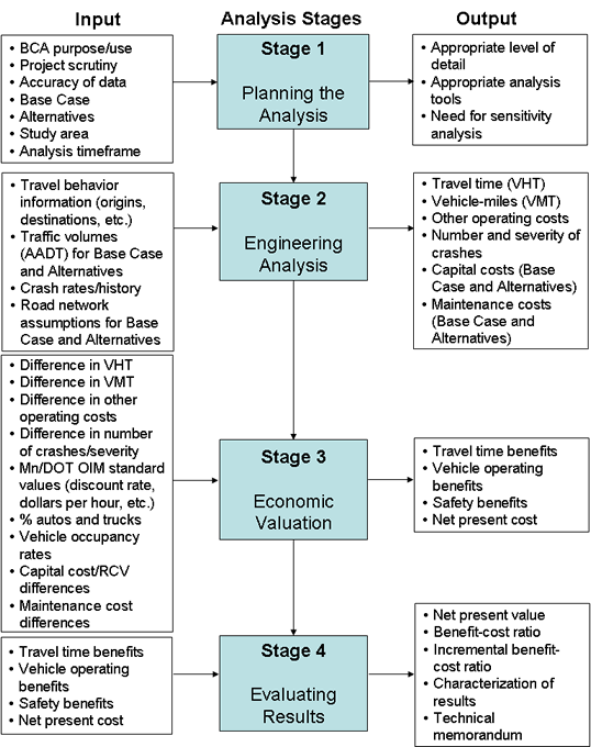
Planning the benefit-cost analysis and performing the engineering analysis (the first two stages) require careful thought. The analysis should capture the appropriate benefits and cost differences between the Base Case and the identified Alternatives. These first two stages are the most complicated and require the most time and effort. The economic calculation stage is a relatively short and straightforward process. Evaluation and interpretation of the results requires judgment and experience. The process of conducting a benefit-cost analysis can be iterative: the process may require going back to a previous stage to verify results and explore sub-alternatives.
The four analysis stages are discussed in more detail below.
5.1 STAGE 1: PLANNING THE ANALYSIS AND DEFINING ITS SCOPE
A successful benefit-cost analysis produces credible results at a level of detail that is appropriate for its intended use and the project’s level of scrutiny. The initial planning activities should define a common framework for comparing the effects of an Alternative against the Base Case. Important elements to define early in the analysis process include the highway scenarios to be analyzed, the start and end years for the analysis, the geographical area considered, and the approach that will be used to analyze travel behavior. It is essential that all alternatives be developed and analyzed to the same level of detail; this should be accounted for in the planning stage. A common framework can be established by completing the following three steps:
1. Define the purpose of the analysis and the appropriate level of detail.
A first step in establishing a framework for the analysis is to define the purpose of the benefit-cost analysis. Will results from the analysis be used to choose between alternatives? Is the analysis being done to show that the Preferred Alternative is economically feasible for inclusion in the final environmental documentation? Or is the analysis being done to test programming scenarios? Identifying the purpose of the analysis helps to define the level of detail appropriate for the study.
Two other factors also help define the appropriate level of detail: available data and analysis budget. Available data varies by project and influences the level of detail appropriate for the benefit-cost analysis. Data sources range from traditional engineering methods to sophisticated regional travel demand models. The availability of this data varies with each project. Benefit-cost analysis planning should establish what data is available, and then verify that the available data suits the analysis purpose and provides the appropriate level of detail for the benefit-cost analysis. The analysis budget influences the appropriate level of detail as well. The level of detail should be consistent throughout the analysis (the same for the Base Case and Alternatives) and commensurate with the available budget.
Figure 4 below shows the relationship between level of data and level of analysis. In the event that the available data lacks the desired level of detail for a scrutinized project, a sensitivity analysis should be considered.
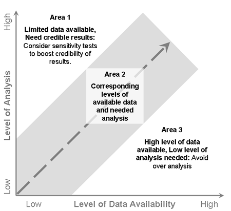
Many times, uncertain data such as travel time or operating costs are given as a range. Sensitivity analyses can be used to test the robustness of benefit-cost results by analyzing the effect that the range of uncertain data has on the final benefit-cost ratio. Analysis planning should include time and resources for sensitivity analyses. A well-planned analysis will produce credible results consistent with the purpose of the analysis and available data issues and budget.
2. Define the base case, proposed alternative and corresponding study area.
Every analysis requires a definition of the Base Case and Proposed Alternative(s). The Base Case is not necessarily a "do nothing” alternative, but it is generally the “lowest” capital cost alternative that maintains the serviceability of the existing facility. In other words, the Base Case should include an estimate of any physical and operational deterioration in the condition of the facility and the costs associated with the periodic need to rehabilitate the major elements of the facility through the analysis period.
The Proposed Alternative(s) are a specific and discrete set of highway improvements that can be undertaken. These improvements generally change travel times, vehicle operating costs, and/or safety characteristics from the Base Case. Proposed alternatives must also be reasonably distinct from one another, i.e., slight alignment shifts or changes that have little to no impact on travel times, safety, or operating costs need not be considered as separate alternatives from the benefit-cost analysis standpoint. The Alternative should be specified in as much detail as possible for purposes of estimating costs (capital and maintenance) and effects on travel time, operating costs, and safety.
An appropriate study area should be chosen so that the majority of the effects of the project are included. The study area should be the logical geographical area within which travel will be affected by the investment Alternative(s) to a material degree.
Benefits of a project are derived from comparing the Base Case highway user data (travel time, operating costs, and safety) that occur within the study area to those of the Alternative scenario(s).
3. Define the analysis timeframe and pertinent years.
Every benefit-cost analysis includes time-dependent elements that must be defined and held consistent throughout the analysis. These elements are:
- Analysis timeframe
- Years of construction
- First year of benefits
- Final year of analysis/year of remaining capital value (RCV)
- Number of days in a year
Figure 5 depicts the different years used. The following text defines the relevant elements and gives typical values where applicable.
Timeframe
The analysis timeframe is the period of time for which project benefits and related costs are compared and evaluated. The general principles for selecting an analysis period are:
- The timeframe should be long enough to capture the majority of benefits, but not so long as to exceed capabilities to develop good traffic information.
- The analysis timeframe should be consistent with that used for other analyses being under-taken for the project, such as transportation demand fore-casts or life-cycle cost models.
- The timeframe should be consistent for all alternatives.
- All benefits and costs occurring or accruing over this timeframe should be included in the analysis.
An analysis period of 20 years is typical for transportation improvement projects, because traffic and demographic information is generally available for this timeframe.
Years of Construction
Construction costs in a benefit-cost analysis are assigned to the year or years in which they are anticipated to occur. If the timing of incurred costs is not known, the construction cost should be divided evenly over the years of construction. For example, if construction is scheduled to last three years, 2001 to 2003, the cost of construction should be divided evenly between the years 2001, 2002, and 2003. Construction costs are then discounted to the year of analysis (defined in Economic Terms and Principles: Discounting).
First Year of Benefits
The first year of benefits is the first full year after construction of the Alternative is complete. For example, if construction is scheduled to be complete in fall 2005, the first year of benefits is 2006.
Final Year of Analysis/Year of Remaining Capital Value (RCV)
The final year of analysis and year of remaining capital value are the same. For example, if the study has a 20-year benefit-cost analysis (2001 to 2020), the final year of analysis and year of remaining capital value is 2020.
- The final year of analysis is defined as the final year of the benefit-cost analysis.
- The year of remaining capital value is defined as the year in which the remaining capital value (salvage value) of a transportation investment is assessed. Methods for calculating the remaining capital value are discussed under “Calculations” (item 6 in Section 5.3).
Number of Days in a Year
The number of days in a year over which benefits accrue depends on the traffic characteristics and the proposed improvement. A typical capacity improvement done in an area with a high-level of commuter traffic (trips between home and work) should use 260 days, the number of weekdays (Monday through Friday) in a year. Weekday effects for this example are chosen because traffic volumes are consistently highest at these times throughout the year. However, if this same example were used with the improvement being a new roadway that reduced trip length for all users by two-miles, benefits would accrue over the 365 days in the year. Also, substantial benefits may occur on weekends for projects in some areas (especially where recreational trip patterns exist). In these cases, weekend benefits can be assessed separately and added to the weekday analysis. In areas with lower commuter volumes, 365 days should be used. The number of days assumed in a year should always be noted in the analysis documentation.
5.2 STAGE 2: ENGINEERING ANALYSIS
Once the benefit-cost analysis is planned, data needs to be assembled and/or generated for the Base Case and the Alternative(s). Data used in MnDOT benefit-cost analyses can be obtained from several engineering sources: field data collection activities, MnDOT’s Traffic Office, project-level travel/traffic modeling results, other general engineering approaches, and professional judgment.
The engineering analyses are alternative-specific and often require a substantial amount of effort. Data produced during the engineering analyses (for the Base Case and Alternative(s) include:
- Benefit-related data
- Average annual daily traffic volumes (AADT)
- Daily vehicle-hours traveled (VHT)
- Daily vehicle-miles traveled (VMT)
- Other operational changes such as daily number of stops of speed-cycle changes
- Annual number of crashes and severity for the Base Case and predicted change(s) to number of crashes and severity based on improvement Alternative(s)
- Cost-related data
- Capital costs
- Annual maintenance and rehabilitation costs
A. Benefit-Related Engineering Analysis
Decisions about appropriate level of detail made while planning the benefit-cost analysis become important when generating benefit-related data. The appropriate level of detail helps define the tools and methods that should be used. Regardless of the tools and methods used to generate data, the analysis should maintain a consistent base (e.g., model base, travel-time base route, etc.) and level of detail for all alternatives.
Several tools and methods can generate traffic volumes (AADT), travel-time (VHT), and vehicle-mile (VMT) data for benefit-cost analyses. Tools and methods include regional travel demand models, local operations models, and engineering judgment and other methods. The appropriate tools and methodologies depend on the study area and Base Case defined during analysis planning. Figure 6 shows project traits and typical tools/methods. In cases where the most typically-used tool is not available, a combination of tools can be used. For example, a regional travel demand model may be used for VMT/VHT information, but a local traffic operations model may be used to estimate the number of speed-cycle changes.
When generating travel-time and vehicle operating data, it is important to account for VHT or VMT changes both on the highway being studied and in the highway system affected by it. For example, one alternative may add a lane to the study highway, which results in an increase in vehicle-miles traveled on the highway facility itself (i.e., attracts trips into the study corridor). However, the new lane may lead to a decrease in the number of vehicle-miles traveled on other facilities in the area. Regional travel demand models are useful for estimating traffic diversion effects. If a regional travel demand model is not available, and significant traffic diversion is likely, traffic shifts should be estimated using other methods such as route diversion curves and travel time estimates.
Travel-Time Data
Travel-time data (vehicle-hours traveled—VHT) is often generated using travel demand models (e.g., TRANPLAN or TP+) or traffic operations models (e.g., Synchro/SimTraffic, CORSIM), by making measurements of existing (Base Case) travel times and adjusting them for the Alternative(s), or using general engineering approaches and judgment. Travel demand models are the primary source for producing VHT data for large projects. They are best suited for analyzing system-wide impacts of various alternatives. Traffic operations models can produce peak hour VHT data for smaller, localized improvement projects. It is important to convert VHT information from peak hour into daily VHT information when using a traffic operations model. For a very simplistic approach, AADT can be converted to VHT by multiplying the AADT by the estimated time needed to travel the corridor in the Base Case and the Alternative(s).
Vehicle Operating Data
Vehicle operations typically include miles traveled and number of stops or speed-cycle changes. (Although idling costs and grade changes could also be evaluated, among others.) The number of vehicle-miles traveled should be forecast for the Base Case and the Alternative(s) using the usual range of engineering tools and methods, often similar to those used to estimate travel time savings. AADT can be converted to VMT by multiplying the AADT by the estimated distance traveled in the corridor in the Base Case and Alternative(s). When hand-calculating this, it is important to capture all of the significant traffic diversions (route changes) as part of this calculation. If using a peak-hour model, estimates of miles of travel should also be converted from peak hour to daily values. To do this, the analyst must understand the travel behavior for the peak hour and relate this to a daily basis.
Vehicles affected by additional stops must go through a speed-cycle change (traveling at posted speeds, braking to stop, restarting and accelerating to posted speed). The number of stops or speed-cycle changes can be estimated using traffic operations models or general engineering approaches and judgment, for example estimate the proportion of daily traffic stopped by a signal. If using a peak hour traffic operations model, stops must be converted to a daily basis.
Safety Data
The safety analysis results in the number of crashes expected for each severity type (fatal, type A injury, type B injury, type C injury, and property damage only). These estimates are made for the Base Case and the Alternative(s) for the first year of benefits and the final year of analysis. The numbers are estimated based on existing and anticipated future crash rate, severity rate, and AADT or VMT.
The crash rates and severity used in the safety analysis should reflect the level of detail appropriate for the benefit-cost analysis. Crash rates and severity are given for different facility types (freeway, expressway), for specific corridors, and for specific sites (roadway segments or intersections). The analyst must determine if the safety analysis should be system-level, corridor-specific, or site-specific based on the Alternative(s) proposed. System-level analyses are appropriate for projects that cause traffic to shift between facility types. Corridor-specific analyses are appropriate when improvements cover a larger area but traffic patterns are anticipated to remain the same. Site-specific analyses are fitting when improvements are site-specific and do not change traffic patterns. The level of detail used in the safety analysis should be consistent for the Base Case and Alternative(s).
Existing crash rates and severity are used for all Base Cases, and for the Alternative(s) in system-level safety analyses and corridor-level analyses where the facility-type changes. System-level safety analyses typically use existing crash rates and severity (historical averages) available from MnDOT District Traffic Engineering office (for roadways under MnDOT jurisdiction) for different facility types. In this case, the forecast AADT or VMT data should be given for each facility type (e.g., freeway or non-freeway). Safety impacts will be evident by the change in AADT or VMT per facility-type throughout the system. Some corridor-level analyses include a facility-type change between the Base Case and the Alternative(s). Safety impacts will be evident if the corridor’s facility-type, and therefore the crash rate and severity rate, changes.
For corridor-level analyses where the facility-type does not change, and in site-specific analyses, Hazard Elimination Safety (HES) tools can be used to estimate reduction in crashes and/or severity. A worksheet aiding in the calculations is available from MnDOT at: http://www.dot.state.mn.us/trafficeng/safety
It is important to remember that all numbers (VHT, VMT, number of crashes, etc.) are needed for each year in the study timeframe. VHT, VMT, and crash data are often generated only for one or two years (e.g., base year and final year of analysis) of the study timeframe and these results are then interpolated/extrapolated for other years in the analysis timeframe.
Figure 7 illustrates data interpolation.
B. Cost-Related Engineering Analysis
Construction costs and maintenance costs should be generated or gathered during the engineering analysis stage of the benefit-cost analysis. Cost estimates should be appropriate for the stage in the project development process. Maintenance costs should include routine maintenance (e.g., plowing, debris removal, etc.) and periodic rehabilitation (e.g., mill and overlay).
Roadway rehabilitation costs for the Base Case should consider the type and extent of pavement distress and the rate of deterioration due to the level of traffic volumes using the facility. The rehabilitation schedule used in the benefit-cost analysis for the Base Case should be based on MnDOT’s Pavement Management System recommendations or on recommendations from the District Maintenance Engineer. Rehabilitation costs for other roadway components, such as bridges, should be evaluated separately and approved by the District Maintenance Engineer.
The Alternative(s) usually involve new construction and include only routine maintenance. A 20 year benefit-cost analysis typically assumes no rehabilitation costs under new-construction Alternative(s). If the benefit-cost analysis timeframe is longer than 20 years, refer to the rehabilitation schedules listed in the MnDOT Pavement Selection Process (Technical Memorandum No. 04-19-MAT-02).
C. Improvements with the Most Effect
When obtaining initial benefit-cost results or considering which alternatives have the greatest impact, the overall traffic volume affected by the alternative should be considered. Changes that affect all traffic generally result in more benefit than changes that affect only portions of the traffic. For example, capacity improvements generate benefits only during times when the facility is congested. If congestion is limited to a few hours (peak hours), then capacity improvements will affect only a small portion of the daily users. Table 1 gives additional examples by listing types of highway improvements and the potential level of daily traffic affected.
Table 1 Traffic Affected by Highway Improvements
| Highway Improvement | Amount of Daily Traffic Affected |
| Adding lanes to a facility that is congested during peak hours | Peak-period fraction of daily traffic |
| Removing a traffic signal (mainline free-flow) | Depends on percentage of mainline green time (30 to 50 percent of daily traffic) |
| Changing the speed limit | All traffic traveling at the speed limit |
| Selecting an alignment that reduces trip length | All traffic traveling on the new facility |
As the alternatives are analyzed, results should be tested for their reasonableness, when compared to the potential volumes impacted (for example, cumulative changes in travel time as compared to the traffic impacted). If results seem out-of-step with impacts, the assumptions and analysis methods should be reviewed.
5.3 Stage 3: Economic Valuation
Highway improvement projects are generally those projects that correct safety, capacity, or system deficiency problems. Once physical benefits have been determined (Stage 2), they need to be monetized and aggregated for the analysis period. The economic valuation also includes estimating the capital cost, maintenance cost, and remaining capital value. A spreadsheet has been developed to aid in the economic valuation calculations. The spreadsheet helps simplify calculations and organizes the results. But before experimenting with the spreadsheet, it is helpful to understand the basic steps in the economic valuation stage of a benefit-cost analysis. Economic valuation consists of two parts: (A) highway user benefit calculation, and (B) cost calculation. The two parts of valuation are described in detail below.
A. Highway User Benefit Calculation
There are four steps in calculating total highway user benefit:
1. Assemble highway user data (VMT, VHT, other operating costs, and safety information) for the first year of benefits and the final year of analysis at a minimum. If detailed annual estimates are not available, interpolate between these two data points to compute information for each year in the analysis timeframe (the spreadsheet aids in this calculation). Data generation and interpolation must be done for the Base Case and the Alternative(s). Table 2 shows a calculation table with VHT data in columns A and B. A calculation table like this should also be prepared for vehicle operating costs, one for vehicle-miles traveled and one for speed-cycle changes, and safety.
2. Compute the difference in travel time, vehicle operating costs, and safety between the Base Case and the Alternative for each year in the analysis. Table 2 shows an example of the difference for VHT in column C. Figure 8 also depicts this difference and shows the difference is the benefit of the Alternative as compared to the Base Case.
Compute the total benefit for travel time, vehicle operating costs, and safety accrued during the analysis timeframe. Total benefit is calculated as follows:
- Find the annual savings for each year in the analysis period. Annual savings are found by multiplying the difference in travel time, vehicle operating costs, and safety by the number of days in the analysis year (may not be applicable for safety), and then multiplying by the appropriate unit cost (e.g., dollars per person-hour traveled, dollars per vehicle-mile traveled, dollars per speed-cycle change, or dollars per crash) for each year in the analysis period. This should be done for each year in the analysis timeframe. Travel-time unit costs should reflect the percent autos and trucks, auto occupancy in peak and off-peak periods, and value of time per person for autos and trucks. The analyst should use vehicle occupancy data collected for the project area or corridor, for example through origin-destination studies. If none is available, Table 3 lists auto occupancy data for different areas of Minnesota. Vehicle operating unit costs should include percent autos and trucks and variable operating costs for autos and trucks. Crash costs should account for crash severity. Use the values of time, variable operating costs, and costs for each crash severity provided by MnDOT OIM (Table A.1 in Appendix A). Annual benefit is shown in column D in Table 2
- Discount the annual benefits back to the year of analysis. This should be done for travel time, vehicle operation costs, and safety for each year in the analysis timeframe. The present value of annual benefits is shown in column E in Table 2.
- Find the overall savings for travel time, vehicle operating costs, and safety by summing the present value of the annual benefit for each year in the analysis timeframe. Table 2 shows the overall travel time savings in the bottom row, column E.
| Table 3: Occupancy Rates | |||
| . | Peak/Off-Peak/Overall |
||
| Automobile Occupancy Rates, Minneapolis-St. Paul (a) | (No Statistical Difference) |
||
| Seven-County Metro Area | 1.30 |
||
| Automobile Occupancy Rates, Greater Minnesota (b) | Urban |
Rural |
Overall |
State-wide Average |
1.68 |
1.52 |
1.64 |
| . | |||
| (a) Source: 2010 Metropolitan Council Travel Behavior Inventory (TBI) Home Interview Survey | |||
| (b) Source: 2017 National Household Travel Survey (NHTS), Minnesota data | |||
| . | |||
3. Find the total user benefit of the Alternative(s) as compared to the Base Case by summing the overall savings for travel time, vehicle operating costs and safety. Table 4 shows an example spreadsheet tallying total highway user benefit. This is the final step in calculating the total highway user benefit.
B. Cost Calculation
There are five steps in calculating agency cost:
1. Construction costs for the Proposed Alternative should be estimated and allocated to the anticipated year of expenditure. If the timing of expenditures is not known, the construction cost should be divided evenly over the years of construction. Discount the construction costs from the year(s) of anticipated expenditure back to the year of analysis. If the Base Case has construction costs, those should be allocated to the year(s) of anticipated expenditure and discounted as well.
2. Maintenance costs for each year should be estimated if an alternative has a significant effect on maintenance costs. Start by estimating the cost of maintenance incurred in each year of the analysis timeframe. This should be done for both the Base Case and the Alternative(s).
3. The constructed infrastructure typically retains some value at the end of the benefit-cost analysis period. This value is called remaining capital value (see definition of RCV, Section 4.2) and it is evaluated at the end of the analysis period (in the final year of analysis) and discounted to the year of analysis.
When calculating remaining capital value, first estimate the useful life of the investment elements (see Table 5). The capital cost should be broken into elements such as preliminary engineering, right-of-way, major structures, roadway grading and drainage, roadway sub-base and base, and roadway surface. Right-of-way costs can include the cost of land and buildings. The useful life of the land and buildings should be considered separately. Table 5 shows that the useful life of land is 100 years; however, the useful life of an acquired building is dependent on if it will be demolished as part of the highway improvement, or if it will be resold. Buildings that will be demolished have a useful life of zero years. The useful life of a building that will not be demolished is the same as the useful life of land (100 years).
After determining the useful life, calculate the percent of useful life remaining at the final year of analysis (see Table A.2 in Appendix A). Multiply that percent by the initial construction cost and discount that amount back to the year of analysis. If the Base Case involves capital expenditures, the remaining capital value should be calculated for the Base Case as well.
1. Find the total present cost for the Base Case and Alternative(s). Table 6 shows the total present cost as the sum of the discounted annual costs found for each year in the analysis timeframe. Annual costs are calculated by adding the construction and ongoing maintenance costs, and subtracting the discounted remaining capital value for each year in the analysis.
PV(Costs) |
= |
PV(CostALT) – PV(CostBASE) |
PV(x) |
= |
Present Value of x |
5.4 Stage 4: Evaluation
The result of the benefit-cost analysis can be shown as benefit-cost ratio and/or as net present value. These results show if the Alternative is economically justified compared to the Base Case. When multiple alternatives are being considered, an incremental benefit-cost ratio analysis can be used to determine which Alternatives are the most economically desirable. Each evaluation method is described below.
Benefit-Cost Ratio
After the future streams of costs and benefits are discounted, the sum of the discounted benefits is divided by the sum of the discounted cost. This can be represented by the following formula:
B/C |
= |
PV(Benefits) |
PV(Costs) |
= |
Present Value of x |
B/C |
= |
Benefit-cost ratio |
PV(x) |
= |
Present Value of x |
If the result is greater than or equal to 1.0, the infrastructure improvement is economically justified.
Incremental Benefit-Cost Ratio
If more than one alternative is considered for a single project, an incremental benefit-cost ratio can be used to determine which Alternative(s) are the most economically desirable (optimize additional benefits gained for the added cost). This can be represented by the following formula:
IB/C |
= |
|
IB/C |
= |
Incremental benefit-cost ratio |
= |
Change in the present value of x (between two Alternatives) |
This is also called the “Challenger-Defender Method.” Alternatives are ordered from least expensive to most expensive. The analysis begins by taking the first two alternatives, the less expensive Alternative is called the “defender” and the more expensive alternative is called the “challenger.”
The change in net benefits between these two alternatives is divided by the difference in net costs. If the result is greater than or equal to 1.0, the increase in benefit of the “challenging” Alternative is equal to or greater than its increase in costs and the “challenger” then becomes the “defender” and is compared to the next Alternative. If the result is less than 1.0, the current “defender” is retained and the new “challenger” becomes the next Alternative on the list. Comparisons of the challenger to defender are made until all Alternatives have been considered. The surviving defender is the most economically efficient.
Net Present Value
All costs and benefits in future years are discounted to the year of analysis using the adopted discount rate. The future stream of discounted costs is subtracted from the future stream of discounted benefits. This can be represented by the following formula:
NPV |
= |
Net Present Value |
PV(x) |
= |
Present Value of x |
If the sum of the discounted benefits is greater than the sum of the discounted costs, the net present value is positive and the infrastructure improvement is deemed to be economically justified.
6 Questions
If you have any questions concerning the processes discussed in this guidance or encounter a situation not specifically covered herein, please call John Wilson at 651-366-3732 or send email to john.wilson@state.mn.us.
Benefit cost analysis of transit projects should be performed using the methodology described in Transit Cooperative Research Program Report 78, Estimating the Benefits and Costs of Public Transit Projects: A Guidebook for Practitioners, Transportation Research Board, 2002
Benefit cost analysis of airport projects should be performed using the methodology described in FAA Airport Benefit-Cost Analysis Guidance, Federal Aviation Administration, December 15, 1999.
Footnotes
- A speed-cycle change is the process of going from the posted or cruising speed to a stop and then back to the initial speed. In this process, additional operating costs for braking and accelerating are incurred.
- The standard crash values are based on value of single life recommended by the US DOT adjusted to include other costs related to crashes. The standard values also account for all of the injuries involved in a typical crash type. For example, most times in Minnesota, more than one person is involved in a fatal crash. The standard crash values account for the average cost of all injuries per crash. The injury statistics are based on the three most recent years of Minnesota crash data.